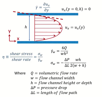
Viscosity is a calculated property and not directly measured. The equations used to calculate viscosity are derived based on specific assumptions. When the assumptions used to perform the viscosity calculation are violated (or wrong), you encounter errors called “data artifacts”, and the value provided by the instrument is flawed. Different artifacts can be observed when using different instruments, and commonly observed artifacts when measuring viscosity with a rectangular slit flow are:
- Turbulence
- Wall slip
- Yielding
- Shear induced heating
- Other inhomogeneities
When measuring viscosity with a rectangular slit flow, the flow rate is controlled, and pressure drop is calculated to determine steady shear viscosity of your sample.
One common assumption relevant to rectangular slit artifacts is unidirectional, or laminar flow. This assumption is that fluid is moving through the flow channel in one direction. This assumption does not account for turbulence or secondary flows. The onset of secondary flows depend on the geometry of your flow channel. These “turbulence” data artifacts are more prone to occur in extensional flow channels due to the geometry of the channel. You are able to adjust for these artifacts using Reynolds number which will predict the transition from laminar to turbulent flow.
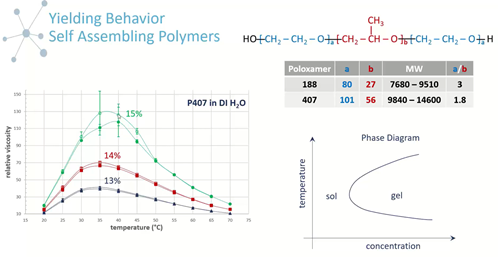
Another common assumption when measuring fluid flow through a rectangular slit channel is the assumption that there are no boundary slip conditions. We measure our fluids viscosity with the assumption that the fluid has zero viscosity at the solid boundaries (or two walls) of our microfluidic flow channel. You are able to account and correct for this data artifact by first getting viscosity and shear rate measurements across a variety of channel depths. Once you have these measurements you are able to apply the commonly used Weissenberg-Rabinowitsch-Mooney (WRM) shear rate correction for non-Newtonian fluids, which will account for wall slip in a rectangular slit channel.  The last common assumption we are going to mention is the assumption that your sample is homogenous in composition and temperature distribution. Some materials, such as polymers, are common “yielding” materials. Yielding samples will move into different phases at different temperatures and concentrations. Below is an example of a poloxamer that self-assemble in solution because the midblock, containing an extra ethyl group is more hydrophobic and will self-assemble.
You can account and correct for these yielding materials using transient curves. These curves look at stress as a function of time, looking to the point where you get to a steady state, then using an average over time to calculate the viscosity of your sample. When dealing with yielding materials you typically see a stress overshoot, which you can also look for in your transient curves to correct for yielding.
The data artifacts we’ve covered are just a few common examples of artifacts that you may observe when measuring viscosity with a rectangular slit flow. Other data artifacts you may encounter include shear induced heating and other inhomogeneities. If you want to learn more about what to look out for and how to handle it if it does occur download our webinar recording “Rheology Tools: Identifying, Understanding, and Handling Data Artifacts” or contact us to speak with one of our rheology experts!
Written by: Eden Reid, RheoSense Senior Marketing Associate


